Excel 2013 v1.0
Question 1
Insert a row.
Directly below current row 1.
Answer : Use the following steps to complete this task in explanation:
Explanation:
Step 1: Open the correct worksheet (Section 3 Worksheet)
Step 2: Click on a cell in row 2.
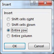
Step 3: Right-click in the cell, and select Insert from the context menu.
Step 4: In the Insert Dialog box select Entire row, and click OK.
Question 2
Apply a cell style -
Cell range A2:S2 -
Style 40% - Accent3 -
Answer : Use the following steps to complete this task in explanation:
Explanation:
Step 1: Open the correct worksheet (Section 3 Worksheet).
Step 2: Click in cell A2.
Step 3: Press down the Shift key and click in cell S2.
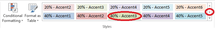
Step 4: On the Home tab, under Format, scroll down until you see 40% . Accent3, and click on it.
Question 3
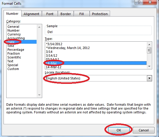
Modify the cell format to date.
Cell range C2:S2 -
Type: 14-Mar -
Locale (location): English (United States)
Answer : Use the following steps to complete this task in explanation:
Explanation:
Step 1: Open the correct worksheet (Section 3 Worksheet).
Step 2: Click in cell A2.
Step 3: Press down the Shift key and click in cell S2.
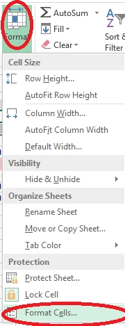
Step 4: On the Home tab, under Format, choose Format Cells.
Step 5: In the Format Cells dialog box, choose Date, 14-Mar, and Locale (location): English (United States). Click OK.
Question 4
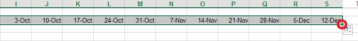
Add a header and the date for each of the columns (assignments) in the range.
Cell B2.
Text "Date".
Cell Range C2: S2 -
Text: "22-Aug, 29-Aug,"¦12-Dec"
Answer : Use the following steps to complete this task in explanation:
Explanation:
Step 1: Click Cell B2. Type the text: Date
Step 2: Click cell C2. Type the text: 22-Aug
Step 3: Click cell D2. Type the text: 29-Aug
Step 3: Click cell C2, then shift-click cell D2.
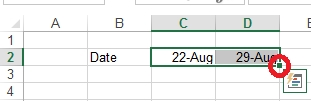
Step 4: Copy until cell S2 (by dragging from cell D2 to cell S2).
Question 5
Modify the text in the title.
Cell A1.
Text "Math 1080 - Section 3 Assignments"
Answer : Use the following steps to complete this task in explanation:
Explanation:
Step 1: Click cell A1 -
Step 2: Change the text by typing to: Math 1080 - Section 3 Assignments
Question 6
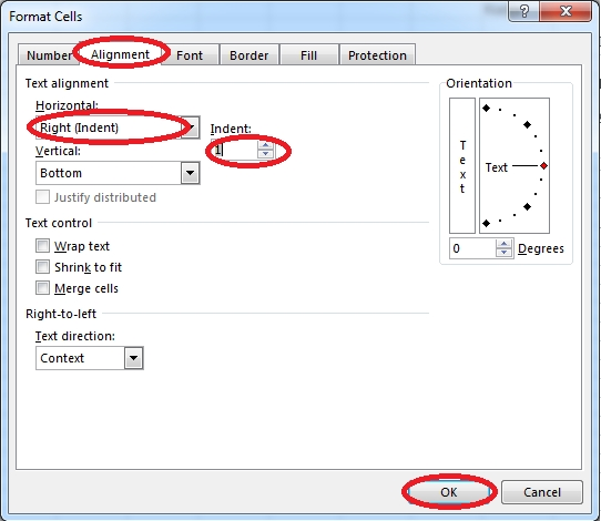
Modify the cell alignment settings.
Cell range B3:B25 -
Horizontal: Right (Indent)
Answer : Use the following steps to complete this task in explanation:
Explanation:
Step 1: Click cell B3.
Step 2:Shift-click cell B25 -
Step 3: Right-click somewhere in the B3-B25 cell range, and choose Format Cells from the context menu.
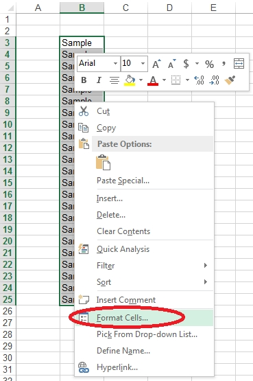
Step 4: In the Format Cells dialog box click the Alignment Tab, change Horizontal: to Right (Indent), change Indent: to 1, and then click the OK button.
Question 7
Add conditional formatting.
Color Scales: Green ""White-Red Color Scale
Midpoint: Percentile, "70"
Maximum: Number, "25"
Answer : Use the following steps to complete this task in explanation:
Explanation:
Step 1: Click cell C3 -
Step 2: Shift-Click cell S25.
Step 3: On the Home tab, under Format, choose Conditional Formatting, and choose New Rule...
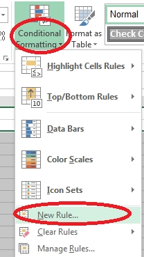
Step 4: In the New Formatting Rule dialog box set Format Style to: 3-Color Scale, and set Minimum Color to Green.
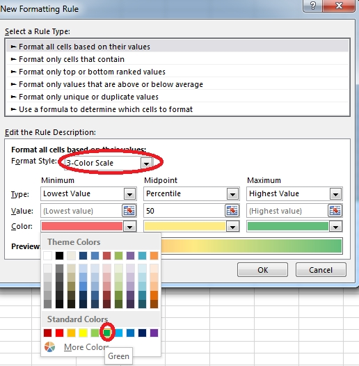
Step 5: In the same dialog box set Midpoint type to Percentile, set Midpoint Value to 70, and set Midpoint Color to White. Also set Maximum Type to Number,
Maximum value to 25, and Maximum Color to Red. Finally click OK.
Question 8
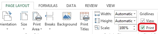
Configure page layout options.
Cell range B3:S25.
Set Print Area.
Enable the Gridlines Print option.
Answer : Use the following steps to complete this task in explanation:
Explanation:
Step 1: Click in cell B3, and then shift-click in cell S25.
Step 2: On the Page Layout tab, in the Page Setup group, click Print Area, and then click Set Print Area.
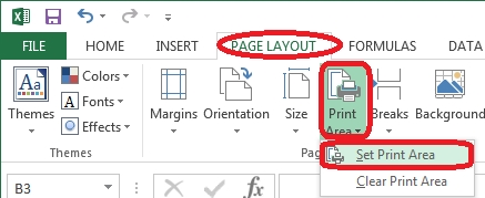
Step 3: Still in the Page Layout tab, Enable the Gridlines Print option.
Question 9
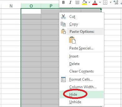
Hide columns.
Column A.
Columns O through R.
Answer : Use the following steps to complete this task in explanation:
Explanation:
Step 1: Right-click on the A column header, and select Hide from the context menu.
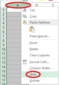
Step 2: Click on the O columns header, and then Shift-click on the R Column Header.
Step 3: Right-click in one of the cells in the high-lighted area, and select Hide from the Context menu.
Question 10
Insert a picture.
To the right of the data -
[1]
Answer : Use the following steps to complete this task in explanation:
Explanation:
Step 1: Click in a cell to the right of the data.
Step 2: Click the INSERT tab, and then the Pictures command.
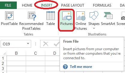
[1]
Question 11
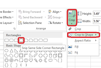
Crop the picture.
[1]
Crop to Shape Snip Same Side Corner Rectangle.
Answer : Use the following steps to complete this task in explanation:
Explanation:
Step 1: Click on the picture.
Step 2: In the Format menu (which is displayed automatically) click the Crop Command, select Crop to Shape, and click Snip Same Side Corner Rectangle.
Question 12
Insert the instructor's name for column B.
Cell B5.
Use Function RIGHT -
Text: B2 -
Absolute reference -
Num_chars: "16"
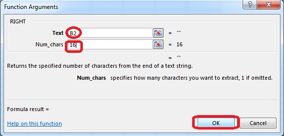
Answer : Use the following steps to complete this task in explanation:
Explanation:
Step 1: Open the correct worksheet (Summary Worksheet).
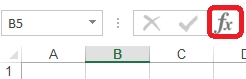
Step 2: Click in cell B5.
Step 3: Click on the insert function button.
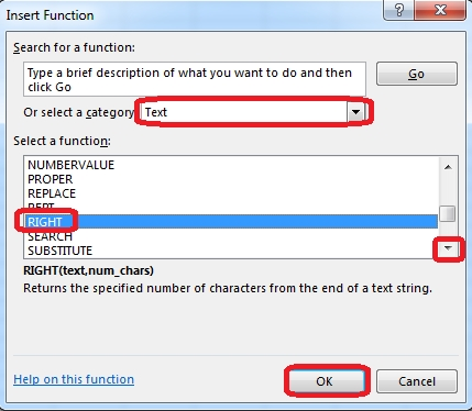
Step 4: In the Insert Function Dialog box select the Category Text, scroll down and click on the function RIGHT, and click OK.
Step 5: In the Function Arguments Dialog box in the Text box type B2, in the Num_chars type 16, and click OK.
Question 13
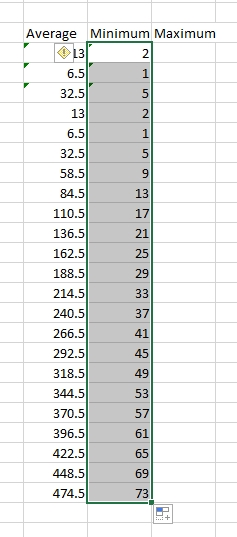
Formula. Find the average of each student's homework scores.
Cell range C7:C29 -
Use Function AVERAGE -
Number 1: all homework for each student on "Section 3" worksheet "22-Aug 12-Dec"
Answer : Use the following steps to complete this task in explanation:
Explanation:
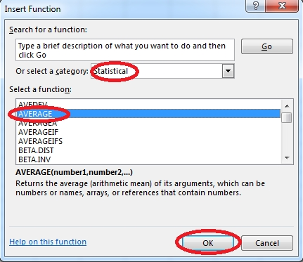
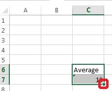
Step 1: Click cell C7, and the click the Insert Function Button.

Step 2: In the Insert Function dialog box select Category Statistical, select function AVERAGE, and click OK.
The function Arguments Dialog box appears:
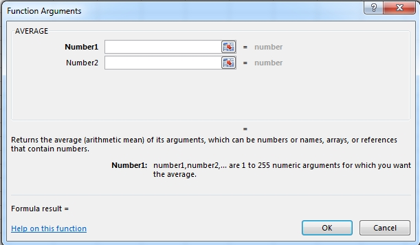
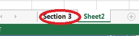
Step 3: Click on the Section 3 tab (left bottom part of the window).

Step 4: Locate the data for the first student. This well be cell range C2 to N2. Click C2 and then Shift-click cell N2. Then click the OK button.
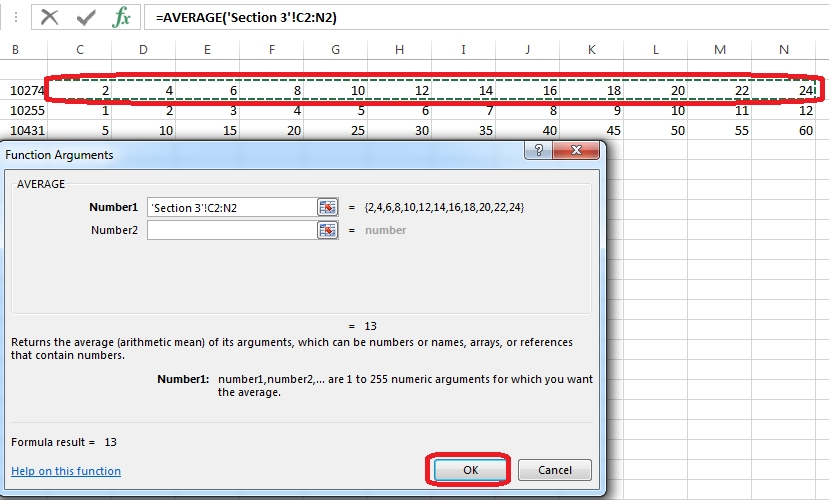
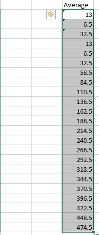
Step 5: Copy cell C7 downwards until cell C29.
Result will be like:
Question 14
Create a new named range.
Cell range C7:C29.
Name: "Homework"
Answer : Use the following steps to complete this task in explanation:
Explanation:
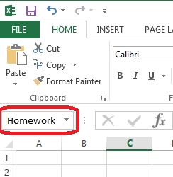
Step 1: Click cell C7, and then Shift-click cell C29
Step 2: Click the Name box at the left end of the formula bar.
Step 3: Type: Homework. Press ENTER.
Question 15
Formula.
Find the minimum homework score for each student.
Cell range D7:D29 -
Number 1: minimum homework score for each student on "Section 3" worksheet.
Answer : Answer:
Explanation:
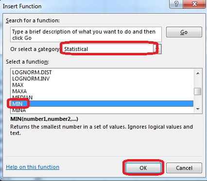
Step 1: Click cell D7, and the click the Insert Function Button.
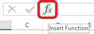
Step 2: In the Insert Function dialog box select Category Statistical, select function MAX, and click OK.
Formula.
Find the minimum homework score for each student.
Step 1: Click cell D7, and the click the Insert Function Button.

Step 2: In the Insert Function dialog box select Category Statistical, select function MIN, and click OK.
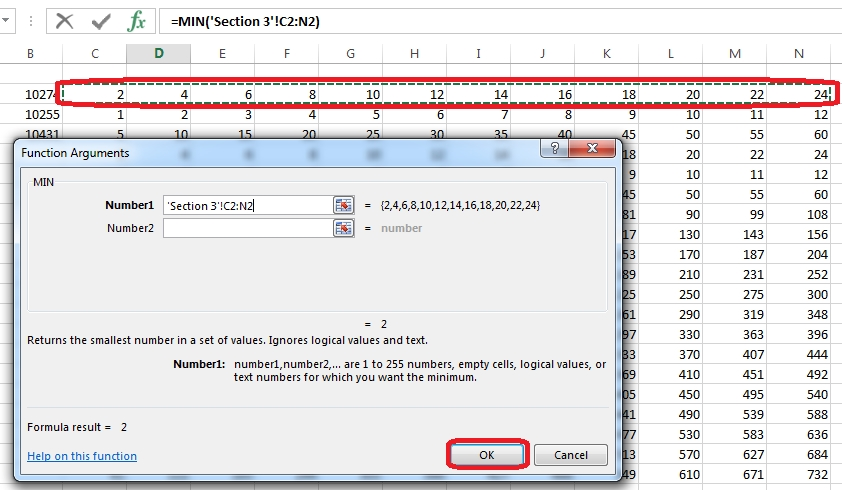
The function Arguments Dialog box appears:
Step 3: Click on the Section 3 tab (left bottom part of the window).
Step 4: Locate the data for the first student. This well be cell range C2 to N2. Click C2 and then Shift-click cell N2. Then click the OK button.
Step 5: Copy cell D7 downwards until cell D29.
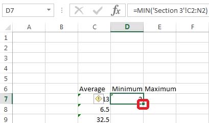
Result will be like: